Building a Spam Classifier from Scratch

Introduction

Spam detection is a classic exercise that presents a solid introduction to machine learning in practice. In this post, we will use some basic tools of natural language processing for sentiment analysis of an SMS dataset from Kaggle. These techniques should allow us to build a system which captures the semantics of each text message and utilize supervised learning algorithms for performance evaluation.

Background

Given our set of text messages, the task is to determine whether each message is spam or not. Our data is a combination of overlapping words/characters/symbols from each message. Our system should learn from the patterns and frequencies provided by the data to establish a baseline for predictions. This can be broken down into several stages.

First, we need to convert our messages into an exhaustive vocabulary list. Next, we will utilize some processing techniques to control for fixed-effects such as part of speech, punctuation, capital letters, etc. This should produce a better signal for our model by reducing the amount of noisy terms. Finally, we will convert our list into a vector where each character sequence will have a corresponding index value.

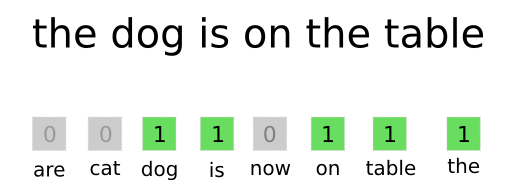
If a message contains a given character sequence from our list, then the corresponding vector index will contain a value of one and zero otherwise. We will effectively transform each message into a vector of ones and zeros indexed by character sequence. All together, the cumulation of these vectors will represent our feature matrix. We will feed this matrix into our algorithms and evaluate its performance. Let’s get started!

Stage One - Building the List

Alright, let’s import our dataset and take care of some cleaning. We’ll drop a few unnecessary columns, rename the ones we’re keeping, and map ‘ham’ and ‘spam’ entries from our target to zeros and ones. Our final preprocessing step is to convert each text message into a list of character sequences, which is also known as tokenizing. All of this work can be done using two python libraries: pandas and nltk. The nltk package provides functionality specific to the natural language processing domain, while pandas is a general platform for data analysis. Let’s have a look at a few tokenized messages.

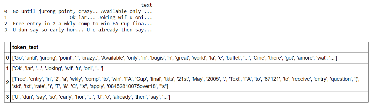
As seen from the image, each message is now a list of character sequences. Here is the small function used for the preprocessing (all code can be found on my GitHub):

def process_spam_data(filepath):
  data = pd.read_csv(filepath, encoding="latin-1")
  data = data[['v1','v2']]
  data = data.rename(columns={'v1':'label','v2':'text'})
  data['label'].replace(['ham','spam'],[0,1], inplace=True)
  data['token_text'] = data['text'].apply(nltk.word_tokenize)
  return data

Stage Two - NLTK Processing

Now we are ready to start building our feature matrix where each row will represent a text message from our training set with ones in columns corresponding to the character sequences in the given message (zeros otherwise). Our goal is to capture as much semantic meaning as possible while maintaining a scalable process with efficient use of computational resources. This dataset contains almost 12,000 unique words and not all return the same signal. Training can quickly become very costly, so we will use some processing techniques to reduce the lower value content.

To start, the NLTK package provides a list of stop words which are a compilation of the most common words observed in text. Stop words provide a lower signal since they are generally observed at a higher frequency. In other words, their semantic meaning changes very little within context. As a result, these words can be safely removed from our list. By simply removing these common words, our list’s length was reduced to about 9800. This is an effective decrease of ~17%. Not bad! Let’s have a look at the top ten stop words removed from our vocabulary list:

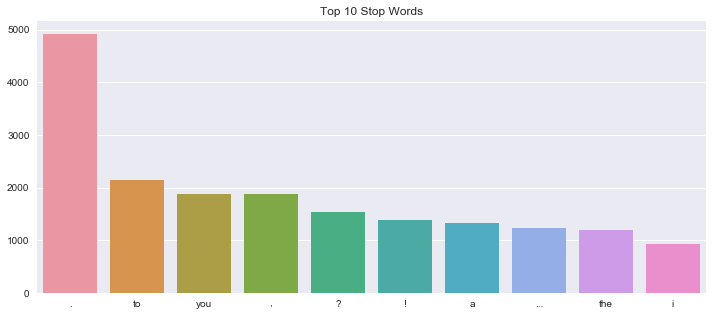
It’s not too surprising to see some pronouns, prepositions, and conjunctions at the top of the list as these parts of speech provide the lowest value in terms of signal. I also added punctuation to the stop-words list (effectively removing punctuation from the dataset).

Next in the process is normalizing our list of terms to their base form. A word can have many representations depending on its part of speech, so we want to reduce these different word endings to the base form, or lemma. NLTK has a class for lemmatization which requires the word representation and its part of speech. I wrote a function to map the nltk tags to the part of speech parameter for the lemmatization class:

def part_of_speech(tag):
    pos = ""
    if (word[1] == 'VB') | (word[1] == 'VBD') | (word[1] == 'VBG') | (word[1] == 'VBN') | (word[1] == 'VBP') | (word[1] == 'VBZ'):
        pos = 'v'
    elif (word[1] == 'RB') | (word[1] == 'RBR') | (word[1] == 'RBS') | (word[1] == 'WRB'):
        pos = 'r'
    elif (word[1] == 'JJ') | (word[1] == 'JJR') | (word[1] == 'JJS'):
        pos = 'a'
    else:
        pos = 'n'
    return pos

This function isn’t the most elegant but it gets the job done. From here, we’ll use our word list to obtain the part of speech tags, use the above function to map the tags to the parameter value for the lemmatization class and finally normalize our word list.

from nltk.stem import WordNetLemmatizer

words = []
for i in data['token_text']:
    words += i
print(len(set(words)))
words = [w.lower() for w in words if w not in stop_words]
tagged_words = nltk.pos_tag(words)

lemmatizer = WordNetLemmatizer()

def lemmatize_words(tagged_words):
    lemmatized_words = []
    for word in tagged_words:
        lemmatized_words.append(lemmatizer.lemmatize(word[0], pos=part_of_speech(word[1])))
    lemma_counts = Counter(lemmatized_words)
    return lemma_counts, lemmatized_words

The end result is a dictionary containing the base representation of each word and its associated frequency. We also get a list of these words for convenience (used later). As a result, the unique set of words was reduced from 9803 to 9286. These basic techniques allowed us to discard ~25% of the low yield content. Pretty sweet! Now what’s left is indexing our vocabulary list and vectorizing our dataset.

Stage 3 - Vectorize the Corpus

The vocabulary list will be indexed from most common to least common. This means the most common word’s index is the 2nd column (index=1), the next most common word’s index is the 3rd column, etc. The first column at index = 0 of the matrix represents the frequency of words not found in the vocabulary due to processing.

def build_common_vocabulary(lemma_counts):
    vocabulary = {}
    index = 1

    for word in lemma_counts.most_common():
        vocabulary[word[0]] = index
        index +=1
    return vocabulary

Let’s now use our lemmatized list to vectorize each message. For each message in our dataset, if each word is in our processed list then we’ll track its frequency in the given message. Next, we’ll index these word counts for each message based on the compiled vocabulary.

Here is the function and resulting output from converting each message to word counts based on our lemmatized list:

text_data = data['token_text']

msg_counts = []
for msg in text_data:
    text = []
    for word in msg:
        word = word.lower()
        if word in lemmatized_words:
            text.append(word)
    word_counts = Counter(text)
    msg_counts.append(word_counts)
print(data['text'].head())
print(msg_counts[:5])

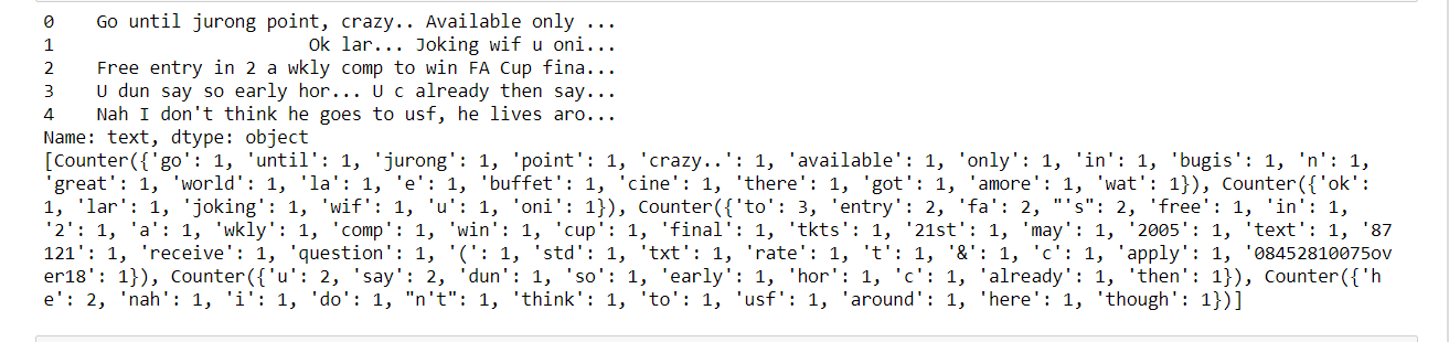
We’re ready to vectorize the text messages using the word counts and vocabulary indices. We’ll use a sparse representation since the matrix will be mostly zeros.

from scipy.sparse import csr_matrix

def vectorize_corpus(msg_counts=msg_counts, vocabulary=vocabulary,
vocab_size=9286):
    rows = []
    cols = []
    data = []

    for row, counter in enumerate(msg_counts):
        for word, count in counter.items():
            rows.append(row)                                     
            cols.append(vocabulary.get(word,0))                  
            data.append(count)                                  
    X = csr_matrix((data, (rows,cols)), shape=(len(msg_counts), vocab_size+1))
    return X

The format of the sparse matrix requires the row and column index for each data entry. These entries are the word counts for a given message. The row index corresponds to particular message and the column index corresponds to a particular word from our global list. If a word is not found in the global list, its count is indexed to column zero. The vectorize_corpus function iterates over the messages, obtains the indices for its word counts, and maps this data to the feature matrix.

Performance Evaluation

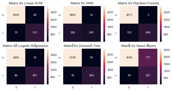
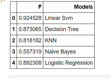
The feature matrix was fed to several supervised learning algorithms for training. Performance was generally strong across the board with f-scores ranging between 0.85 and 0.92 on the training set! Parameter tuning had a strong effect on results, especially for the logistic regression algorithm. High precision and low recall indicated a sub-optimal threshold for its decision function. An increase in performance of more than 50% resulted from simply adjusting its threshold value (Please see the GitHub repository for code).

Here are the confusion matrices and final results for testing: