Convergence of Linear Models

Introduction

This post will cover the techniques and concepts used for training linear models. While most of the information presented here has already been covered elsewhere with great detail, I hope to present it in such a way that is relatable to anyone interested in data science. In doing so, I will also test the depth of my own knowledge and improve my written communication as a result. For additional information, a list of references will be provided at the end of this post.

Background

Supervised learning is a classic domain of statistics which involves a set of features and a response variable. A supervised learning model seeks to capture the full relationship between the features and the response for prediction/inference. If this relationship exists, then there must be some function which relates the systematic information of the features to the response. The modeling process amounts to approximating this function and evaluating the results. The general form of the function can be written in the following way:

$$\begin{equation} Y = f(X) + \epsilon \end{equation}$$

In this equation, $f$ is our model and $\epsilon$ represents the variation of $y$ not captured by our model. Linear models are named as such because they associate a linear shape for $f$. Here is the general form of a linear model:

$$\begin{equation} f(X) = \beta_{0} + \beta_{1}X_{1} + \beta_{2}X_{2} +...+\beta_{n}X_{n} \end{equation}$$

$\beta_{0}$ is a constant term representing the bias for model training. Every other parameter has an associated feature ($X_{1:n}$) representing the measured effect of $X_{i}$ on $Y$. Given some data, we can use this model to make predictions as a weighted sum of the input features. These predictions are evaluated using a performance measure, typically RMSE (Root Mean Squared Error). Here, RMSE is represented using matrix notation where $\theta$ are the model parameters and $X$ is our feature set.

$$\begin{equation} RMSE = ((1/n)\sum_{i=1}^{n}[y_{i}-\theta^{T}X_{i}]^{2})^{1/2} \end{equation}$$

For each instance, we take the squared difference between our prediction and the label, add them up, and normalize the result. It follows that we need to find the best combination of parameters which minimize model errors ($y_{i}$ - f(X)). There are two approaches to accomplish this task.

The Closed Form Solution

In this section, I will go through the steps to find model parameters for a single feature. Applications with multiple features are conceptually the same process but use matrix notation for convenience. In either case, the goal is a direct solution of optimal parameters instead of an iterated approach (more on this later). Lets get started!

Our goal is to minimize our performance measure (RMSE) with respect to the model parameters ($\beta_{0}$ and $\beta_{1}$). We can drop the square root and the (1/m) constant since they have no effect on the end result. This simplifies our function to the squared-sum of model errors (SE):

$$\begin{equation} SE = \sum_{i=1}^{n}(y_{i}-\beta_{0}-\beta_{1}x_{i})^{2} \end{equation}$$

We can obtain a direct solution through partitioning our cost function with respect to each model parameter. First, we’ll take the partial derivative of SE for $\beta_{0}$.

$$\begin{equation} \beta_{0}^{'} = -2\sum_{i=1}^{n}(y_{i}-\beta_{0}-\beta_{1}x_{i}) = 0 \\ = \sum_{i=1}^{n}(y_{i}-\beta_{0}-\beta_{1}x_{i}) = 0 \\ \sum_{i=1}^{n}\beta_{0} = \sum_{i=1}^{n}y_{i} -\beta_{1}\sum_{i=1}^{n}x_{i} \\ n\beta_{0} = \sum_{i=1}^{n}y_{i} - \beta_{1}\sum_{i=1}^{n}x_{i} \\ \beta_{0} = (1/n)\sum_{i=1}^{n}y_{i} - \beta_{1}(1/n)\sum_{i=1}^{n}x_{i} \\ \beta_{0} = \bar{y} - \beta_{1}\bar{X} \end{equation}$$

After dropping the -2 constant, we distribute the summation operator and rewrite in terms of $\beta_{0}$. $\beta_{0}$ is the model intercept, so a summation over a constant also produces a constant ($n\beta_{0}$).

We can now use this result with the partial derivative of SE for $\beta_{1}$ to derive the direct solution.

$$\begin{equation} \beta_{1}^{'} = -2\sum_{i=1}^{n}(y_{i}-\beta_{0}-\beta_{1}x_{i})(x_{i}) = 0 \\ = \sum_{i=1}^{n}x_{i}(y_{i}-\beta_{0}-\beta_{1}x_{i}) = 0 \\ =\sum_{i=1}^{n}x_{i}y_{i}-\beta_{0}\sum_{i=1}^{n}x_{i}-\beta_{1}\sum_{i=1}^{n}(x_{i})^{2} = 0 \end{equation}$$

The result of the partial derivative for $\beta_{1}$ is still in terms of $\beta_{0}$, so we need to do a bit more work. We can use the partial for $\beta_{0}$ as a function of $\beta_{1}$ to substitute and solve for $\beta_{1}$ using some algebra. The end result is a little messy but is a direct solution nonetheless!

$\begin{equation} \beta_{1} = \frac{\sum_{i=1}^{n}x_{i}y_{i}-(1/n)\sum_{i=1}^{n}x_{i}\sum_{i=1}^{n}y_{i}}{\sum_{i=1}^{n}(x_{i})^{2} - (1/n)(\sum_{i=1}^{n}x_{i})^{2}} \end{equation}$ $\begin{equation} \beta_{1}=cov(x,y)/var(x) \end{equation}$

And here is the much cleaner solution in matrix notation for the general case:

$$\begin{equation} \theta = (X^{T} \cdot{X})^{-1} \cdot{X^{T}} \cdot{y} \end{equation}$$

Implementation

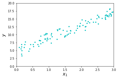
Now that we have a conceptual understanding of the linear regression algorithm, let’s build it! First, we’ll generate some data and plot it. We should expect to see a linear relationship between changes in $x_{1}$ and $y$.

import numpy as np
import matplotlib.pyplot as plt

np.random.seed(11)

X1 = 3*np.random.rand(100,1)
y = 5 + 4*X1 + np.random.randn(100,1)

plt.plot(X1,y,"c.")
plt.xlabel("$x_1$",fontsize=15)
plt.ylabel("$y$",fontsize=15)
plt.axis([0,3,0,20])
plt.show()

As expected, the data reflects a positive association of $x_{1}$ with $y$. $x_{1}$ is an array of 100 data points drawn from the uniform distribution ([0,1)) and $y$ is also an array of 100 data points dependent on $x_{1}$ plus some noise. The noise is randomly generated from the normal distribution, consistent with model assumptions for errors (mean = 0).

Now let’s optimize for our parameters. We’ll account for our model’s intercept by appending a column of one’s to the $x_{1}$ data. In this way, the intercept is implemented the same as any feature but with an input value of one for every instance. Next, we can implement the direct solution with one line of code and numpy! Here are the results:

X0_X1 = np.c_[np.ones((100,1)),X1]
theta = np.linalg.inv(X0_X1.T.dot(X0_X1)).dot(X0_X1.T).dot(y)

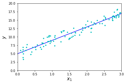
We can visualize our linear model as a function of $x_{1}$ by connecting the prediction results from its fringe values (constant slope). In this case, our data ranges from [0,3] so we’ll compute predictions for these inputs and plot the fitness of our model.

X_fringe = np.array([[0],[3]])
X0_X1_fringe = np.c_[np.ones((2,1)),X_fringe]
y_fringe = X0_X1_fringe.dot(theta)

plt.plot(X_fringe,y_fringe,"b-")
plt.plot(X1,y,"c.")
plt.xlabel("$x_1$",fontsize=15)
plt.ylabel("$y$",fontsize=15)
plt.axis([0,3,0,20])
plt.show()

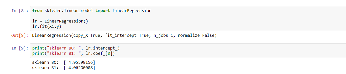
Looking good! Finally, let’s check our implementation vs a packaged version from Scikit-Learn. Our model parameters should be the same as theirs if we didn’t make any mistakes (direct solution).

from sklearn.linear_model import LinearRegression

lr = LinearRegression()
lr.fit(X1,y)

print("sklearn B0: ", lr.intercept_)
print("sklearn B1: ", lr.coef_[0])

Gradient Descent

Consider that the Normal Equation requires computation and inversion of the matrix $(X^{'}X)^{-1}$, which can become expensive and slow as model dimensionality increases. Gradient Descent is another approach to finding the optimal set of model parameters and scales much better with the number of features. It starts with a random initialization of parameter values, and given these values, computes a number of iterative adjustments based on the local optima and the learning rate.

In other words, since our performance measure (MSE) is a function of our model parameters ($\theta$), gradient descent starts with a random set of parameters and incrementally improves the recent set with each iteration. Model training converges to the best set of parameter values when the local optima approximate the global optima with a tolerable level of error.

The learning rate is the pace of adjustment for the parameters based on the local optima and it’s actually an important part of the algorithm. If it’s set too small then training can take an unnecessarily long amount of time, but if it’s too large then it’s possible to miss the set of parameters which minimize model errors. In practice, a learning rate of 0.1 is used as a default.

Partitioning our performance function with respect to a given parameter ($\theta_{j}$) is equal to the following equation:

$$\begin{equation} \frac{\partial}{\partial\theta_{j}}SE(\theta) = \frac{2}{n}\sum_{i=1}^{n}(\theta^{T} \cdot{x^{(i)}}-y^{(i)})x_{j}^{(i)} \end{equation}$$

Given the current values of $\theta$, Gradient Descent computes the partial derivatives for each feature and adjusts $\theta$ based on these local optima and the learning rate. The cumulation of these partial derivatives can be represented as a vector and computed in the following way:

$$\begin{equation} \nabla_{\theta}SE(\theta) = \frac{2}{n}X^{T} \cdot{(X \cdot{\theta -y})} \end{equation}$$

Implementation

Notice that the function for the gradient vector uses the entire dataset for training. This is called Batch Gradient Descent because it uses all of the training data during each iteration of computing the gradients. As a result, training with Batch scales poorly with larger datasets.

The implementation is fairly straightforward.

adj_rate = 0.1
iterations = 1000
n = 100
theta = np.random.randn(2,1)

for iteration in range(iterations):
    gradients = 2/n * X0_X1.T.dot(X0_X1.dot(theta) - y)
    theta = theta - adj_rate*gradients

print("model intercept: ",theta[0])
print("x1 parameter:    ",theta[1])

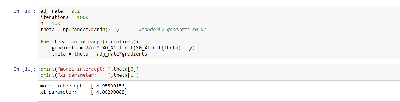
We randomly initialize $\theta$ from the normal distribution (mean = 0) to ensure no directional bias for the gradients, on average. Then we compute the gradient vector for each iteration and adjust our $\theta$ according to the learning rate. As expected, the results are identical for Batch Gradient Descent.

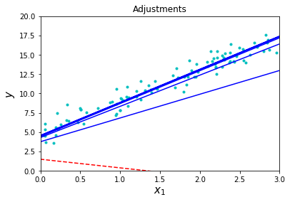
Let’s have a look at the first ten adjustments of $\theta$ using Batch Gradient Descent. The algorithm appears to converge quickly for this dataset. The dashed red line is the random initialization of parameters.

References

1. Hands-On Machine Learning with Scikit-Learn and Tensorflow by Aurelien Geron (O’Reilly)
2. An Introduction to Statistical Learning by Gareth James, Deniela Witten, Trevor Hastie, and Robert Tibshiran (Springer)
3. An Intuitive Introduction to Gradient Descent by Thalles Silva https://towardsdatascience.com/machine-learning-101-an-intuitive-introduction-to-gradient-descent-366b77b52645
4. Derivation proof https://math.stackexchange.com/questions/716826/derivation-of-simple-linear-regression-parameters