Maximum Likelihood Estimation

Introduction

This post will build on a previous one which covered some techniques for convergence of linear models (found here). As a brief review, statistical inference is the process of building a model which reflects the patterns and properties of a given dataset. In the case where the functional form is assumed to be linear, the process conveniently simplifies to computing the set of model parameters which minimize model errors.

For the general case, we need a way to approximate the functional form of the data before computing the model parameters and a common technique used in practice is known as Maximum Likelihood Estimation. We will consider an application of MLE with an implementation of Logistic Regression from scratch.

MLE - Background

The terms probability and likelihood are semantically similar but there is a technical difference in application. First, probability is a measure of outcome where likelihood is a measure of the model. The likelihood function estimates the set of parameter values which maximize the certainty of the observed probabilities. In this way, likelihood quantifies trust in the model, given the data. The formal notation for the likelihood is as follows:

$$\begin{equation} L(\theta;x^{n}) = p(x^{n};\theta) \end{equation}$$

L is the likelihood function. It is the joint distribution of the observed probabilities and is used to estimate the best $\theta$ consistent with these probabilities. It also has some nice statistical properties which allow for easier computation. Assuming the data is a random sample from some probability distribution, we can represent the joint probability distribution as the product of univariate distributions (which are all the same!).

$$\begin{equation} L(\theta;x^{n}) = \prod_{i=1}^{n}p(x_{i};\theta) \end{equation}$$

We can simplify things further by working with the log-likelihood. Since the log function is nondecreasing, the maximum likelihood estimate for the likelihood will be the same for the log-likelihood. This will allow us to convert the product of univariates to a sum of univariates which helps for derivatives. For information on log properties see this link

$$\begin{equation} l(\theta;x_{i}) = logL(\theta;x_{i}) \end{equation}$$

From here, we can use good ol’ calculus to partition l($\theta$;$x_{i}$) for the $\theta$ most consistent with our data. Alright, this stuff is pretty abstract. Let’s put it to the test with an implementation of Logistic Regression.

Logistic Regression - Motivation

Regression models typically estimate the response of continuous variables from a set of fixed variables for prediction and/or inference. Said another way, prediction results are formulated as the conditional expectation of a continuous variable, where we can measure the average value of the input-output relationship. But what if our response is categorical and not continuous? It turns out that linear models can also be used in this instance as well.

Suppose our task is to project the default status of some student loans. It would seem reasonable to assume some randomness in the result of this binary outcome due to the difficulty of projecting 4+ years into a student’s future (among other considerations!). As a result, we will need an associated probability for our projections to account for this noise. Conveniently, for binary outcomes, Pr(Y=1) = E[y] (ratio of 1’s for the response) and Pr(Y=0) = 1-Pr(Y=1).

This means we can use our linear model to project the probability of default and use some threshold rule for loan classification. The issue, however, is the results of our linear model are unbounded and will require a transformation to express the results as probabilities. For this purpose, we can take the log odds of our result, which is the log of the ratio of success/failure. Thus, our model can now be represented in the following way:

$$\begin{equation} log\frac{p(x)}{1-p(x)} = \beta_{0}+X\beta \end{equation}$$

This is known as the logistic regression model. Solving for (p) gives the following result:

$$\begin{equation} p(x) = \frac{1}{1+e^{-(\beta_{0}+X\beta)}} \end{equation}$$

We can take the exponential of both sides to drop the natural log and use a little algebra to solve for (p). The result is known as the logit function. We can use the logit to represent the results of our linear model as probabilities bound by zero and one. We’ll then use these probabilities to classify results and evaluate performance. Here is a visual of the logit function.

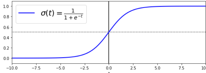
Here, the data is evenly distributed around zero so negative inputs (t) produce probabilities less than 0.5 and positive inputs have probabilities greater than 0.5. The Logistic Regression algorithm for scikit-learn uses 0.5 as a baseline for classification. That is, transformed outputs greater than 0.5 are classified with a label of Y=1 and Y=0 otherwise. Hence, (p) is the probability that Y=1. Finally, we need to optimize our model parameters consistent with the observed probabilities.

Likelihood Function for Logistic regression

Given the iid assumption that the data is a random sample, the likelihood function for Logistic Regression is a product of Bernoulli distributions.

$$\begin{equation} L(\beta_{0},\beta) = \prod_{i=1}^{n}p(x_{i})^{y_{i}}(1-p(x_{i}))^{1-y_{i}} \end{equation}$$

$x_{i}$ is our feature vector, $p(x_{i})$ is the logit, and $y_{i}$ is the observed class for the associated probability of (p). The log-likelihood can be represented in the following way:

$$\begin{equation} l(\beta_{0},\beta) = \sum_{i=1}^{n}y_{i}logp(x_{i})+(1-y_{i})log1-p(x_{i}) \end{equation}$$

We can distribute and combine terms using log properties:

$$\begin{equation} = \sum_{i=1}^{n}log1-p(x_{i})+\sum_{i=1}^{n}y_{i}log\frac{p(x_{i})}{1-p(x_{i})} \end{equation}$$

Using the division property of logs, the first term can be written as (1/logit) = $\frac{1}{\frac{1}{1+e^{-\beta_{0}+x_{i}\beta}}}$, which we can simplify a bit further for easier derivatives. The second term is our Logistic Regression model.

$$\begin{equation} l(\beta_{0},\beta) = \sum_{i=1}^{n}-log1+e^{\beta_{0}+x_{i}\beta}+\sum_{i=1}^{n}y_{i}(\beta_{0}+x_{i}\beta) \end{equation}$$

Now, we need to differentiate the log-likelihood for each parameter ($\beta_{j}$) to find the maximum likelihood estimates.

$$\begin{equation} \frac{\partial}{\partial\beta_{j}} = -\sum_{i=1}^{n}\frac{e^{\beta_{0}+x_{i}\beta}}{1+e^{\beta_{0}+x_{i}\beta}}x_{ij}+\sum_{i=1}^{n}y_{i}x_{ij} \end{equation}$$

After partitioning the log-likelihood for $\beta_{j}$, we’re left with the logit of the jth feature for each observation and the label of the jth feature for each observation. Combining terms gives the following function for the gradients:

$$\begin{equation} = \sum_{i=1}^{n}(y_{i}-p(x_{i}))x_{ij} \end{equation}$$

We will use this function to iteratively update and evaluate our feature set, where performance is the difference between the label and estimated probability given the current set of parameters.

Model implementation

Now, let’s generate some data and train a model!

np.random.seed(88)
m1 = [0,0]
m2 = [2,5]
n = 3000

x1 = np.random.normal(m1,size=[n,2])
x2 = np.random.normal(m2,size=[n,2])

features = np.vstack((x1,x2)).astype(np.float32)
labels = np.hstack((np.zeros(n),np.ones(n)))

Here, we simulate some data and ensure it’s linearly separable from different sample means. Then we combine the data to form our feature set and attach the labels. A plot of the data should clearly distinguish between the two classes. Let’s have a look!

plt.style.use('ggplot')
plt.figure(figsize=(10,8))
plt.scatter(features[:,0],features[:,1],c=labels)
plt.show()

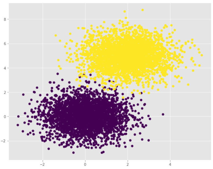
As you can see, we can easily separate this data with a linear decision boundary. Right on! Now that we have our data, let’s build the model. First, we’ll define the logit function, append the model intercept to our feature set, and initialize random values for the model parameters.

# define logit function
def logit(output):
    return 1/(1+np.exp(-output))

# account for model intercept
x0_features = np.c_[np.ones((len(features),1)),features]

# randomly initialize parameters
theta = np.random.randn(3,1)

We’re now ready to build the model. We’ll also need an adjustment rate for the gradient updates and the number of iterations for training. Ideally, training would continue until model error is sufficiently low, but 100,000 iterations will get us close enough. For each iteration, we’ll compute the output from the linear model, transform it to a probability, and compute the gradients from the differentiated log-likelihood function. Training should produce a model which correctly classifies both features with high accuracy.

# Logistic Regression from scratch
adj_rate = .01
iterations = 100000

for iteration in range(iterations):
    #transformation
    linear_output = np.dot(x0_features,theta)
    probs = logit(linear_output)

    #update
    performance = labels.reshape(6000,1) - probs
    ll = np.dot(x0_features.T,performance)
    theta = theta + adj_rate*ll

Alright, so we have a linear model which uses a transformation function and Maximum Likelihood Estimation for classification. Let’s compare our model parameters for Logistic Regression with Scikit-learn’s. The hyperparameter (C) accounts for regularization which we didn’t account for in our model, but could be a topic for a future post!

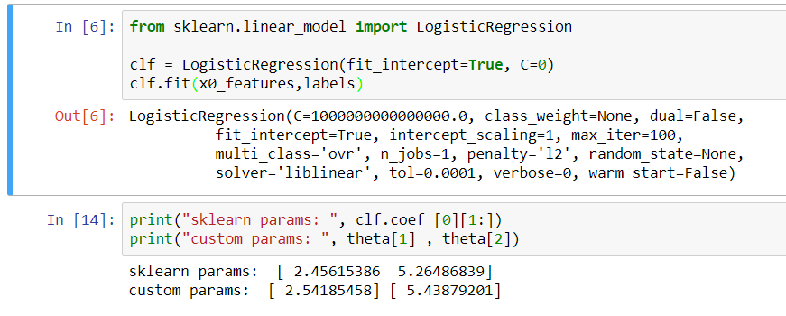
Our model’s parameters are, in fact, very close to the out-of-the-box version from sklearn. Very cool! To consider performance, let’s round the probabilities generated from our model and plot the conditional result of comparison to the labels. So, if the probability rounds to a one and the corresponding label is also a one then the model was correct in its prediction. Correct predictions are the yellow points in the following plot:

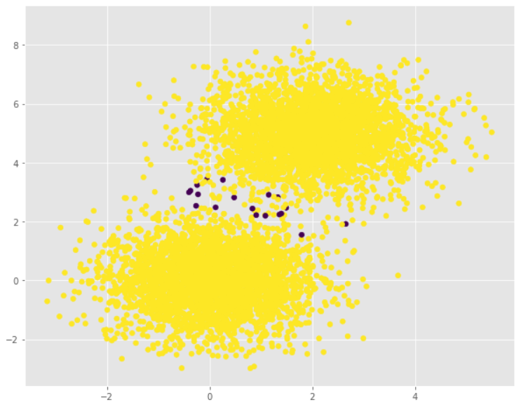
Our model performs very well with over 99% accuracy!